Stability of large random communities

Note: | Most of the theory here is copied and/or derived from this excellent blog post by Stefano Allesina, an amazing ecologist that makes tremendous effort to understand the stability of complex ecosystems. I basically just ported his R-code to Julia.

Large ecological communities can often be captured in a matrix form. This means that the generalized Lotka-Volterra model for $n$ species can be written in a compact form: $$ \frac{dx(t)}{dt} = \boldsymbol{D}(x) \big(r + \boldsymbol{A}x(t) \big), $$ where $x(t)$ the state vector – i.e. the population densities for the $n$ species –, $\boldsymbol{D}$ a diagonal matrix with elements $x_i$ on the diagonal, $r$ a vector of intrinsic growth/decay rates (e.g. reproduction and/or mortality rate, depending on the sign), and $\boldsymbol{A}$ an $n\times n$ matrix of interaction coefficients.

In the interest of the stability of ecological communities we look for solutions where $r + \boldsymbol{A}x(t)$ has positive components. Or, for some $i$, $x_i>0$ when $dx_i=0$. We call this state $x^\dagger$ the feasible equilibrium. Note that if $x^\dagger$ exists that is is unique and the solution of $x^\dagger = -\boldsymbol{A}^{-1}r$. This means that $\boldsymbol{A}$ should have an inverse.

It is often interesting to check whether $x^\dagger$ is an attractor. This problem is in general difficult to solve, so one often tests for local asymptotic stability instead. To do this, describe the evolution of the ecological community as a system of nonlinear ODEs: $$ \frac{dx_i}{dt} = f_i(x) $$ and define the equilibrium as a vector of densities for which the derivative is $0$, i.e. $$ \frac{dx_i^\dagger}{dt} = f_i(x^\dagger) = 0 \quad \forall i. $$ Then, suppose a system is in a feasible equilibrium and we perturb the system at $t=0$, resulting in a change $\Delta x(0) = x(0) - x^\dagger$. Taylor expansion around $x^\dagger$ (and omitting higher order terms) gives $$ f(\Delta x) = f(x^\dagger) + J(x^\dagger)\Delta x + \ldots, $$ where $J\rvert_{x=x^\dagger}$ the Jacobian matrix evaluated at $x^\dagger$ with $J_{ij} = \frac{\partial f_i}{\partial x_j}$. In theoretical ecology, the Jacobian evaluated at $x^\dagger$ is called the community matrix $$ M = J(x^\dagger)\rvert_{x=x^\dagger} $$ This matrix details the effect of increasing the density of one species on any other species around the equilibrium point. Interestingly, as May, 1927 pointed out, random matrix theory shows that the eigenvalues of $M$ determine the stability of the equilibrium $x^\dagger$. In short, if all eigenvalues $\lambda_i$ have negative real parts, then the system will eventually return to $x^\dagger$ after a perturbation. As a result, it suffices to check if the ‘rightmost’ eigenvalue $\lambda_r$ (i.e. the eigenvalue with the largest real part) has a negative real part. If that is the case, then the equilibrium is stable.

Random matrix theory: the distribution of eigenvalues and community stability

Interestingly, the distribution of eigenvalues can be computed for large random communities (i.e communities for which $n\rightarrow \infty$) of which the components of the community matrix are random with mean $0$ and variance $\sigma^2$. While the specific form of the distribution was conjectured for long, the proof for the law is still relatively young (see Tao, Vu, 2010). Here I will highlight the so-called circular law (but see below for the elliptic law) of the distribution of eigenvalues of random communities.

Circular law

For a random $n\times n$ matrix with coefficients $X_{ij}$ random with $\mathbb{E}[X_{ij}] = 0$ and $\mathbb{E}[X_{ij}^2] = 1$, the empirical spectral distribution of $X/\sqrt{n}$ converges as $n\rightarrow \infty$ to

$$ \mu(\lambda) = \cases{ 1/\pi \quad &\text{if} \quad \text{Re}(\lambda)^2 + \text{Im}(\lambda)^2 \leq 1 \cr 0 \quad &\text{otherwise} } $$

This law can be used to compute the radius of the eigenvalue distribution of some community matrices of interest.

On the stability of random communities

In particular, the matrix that May studied is defined as follows. Consider a community matrix $A$ that has elements $A_{ij}=0$ with probability $1-P$ and $A_{ij}\sim p(0;\sigma^2)$ with probability $P$. The diagonal elements are set to $-d$. This gives a matrix of which the elements have mean $0$ and variance $P\sigma^2$. We find the normalized matrix $M = A/\sqrt{P\sigma^2}$ to have unit variance of its random elements. The distribution of eigenvalues of $M$ follows the circular law for $n$ large. The radius of the circle can be computed as we find $A/\sqrt{nP\sigma^2} \rightarrow 1$, thus the radius of the circle wherein all eigenvalues lie is given by $$ R = \sqrt{nP\sigma^2}. $$ Recall that for the equilibrium to be stable we need the rightmost eigenvalue to have a negative real part. In other words, $$ -d + \sqrt{nP\sigma^2} < 0. $$ In May’s case, he defined $d=1$, which leads to his now famous result $\sigma < (nP)^{-1/2}$ for a stable community. From this inequality he notices that if the number of species $n$ is large, then the number of interactions between species (sampled with prob. $1-P$) should be low (i.e. $P$ large), or the variance of the distribution should be small. As a result, he concluded that heterogeneous ecological communities (large $\sigma$) with many members and interactions (high $n$ and $P$) cannot be stable.

Random communities are not ‘just’ random

However, as noted by Allesina, the effect of species $i$ on species $j$ (and vice-versa) are typically not independent (as assumed by May). For example, if two species are competitors, then we expect $X_{ji}$ to be negative if $X_{ij}$ is negative. Another example, if one species consumes another species (predator-prey), then we expect $X_{ji}$ to have an opposite sign than $X_{ij}$. Therefore, a more realistic model of a random community matrix would therefore sample the elements of $M$ from a bivariate distribution instead. In this case, the circular law becomes an elliptic law.

The elliptic law

For a random $n\times n$ matrix in which the pairs of coefficients $(X_{ij}, X_{ji})$ are sampled independently from a bivariate distribution with mean $(0,0)^T$ and covariance $\Sigma = \left(\begin{matrix} 1 & \rho \cr \rho & 1 \end{matrix}\right)$, the empirical spectral distribution of $X/\sqrt{n}$ converges to the elliptic law $$ \mu(\lambda) = \begin{cases} \frac{1}{\pi(1-\rho^2} \quad &\text{if} \quad \frac{\text{Re}(\lambda)^2}{(1+\rho)^2} + \frac{\text{Im}(\lambda)^2}{(1-\rho)^2} \leq 1 \cr 0 \quad &\text{otherwise} \end{cases} $$ (Note that when $\rho=0$ the law converges to the circular law.)

Some code examples

To highlight the truth behind these laws, let us plot the eigenvalue distribution of a few matrices using Julia. For the full code, please check my github repository. Below, let us define some functions that generate three types of matrices: May’s matrix, a competition mutualism matrix, and a predator-prey matrix.

May’s matrix

"Generate a matrix M that follows May's assumptions: 
 1. Elements Mᵢⱼ are 0 with prob. P with i≠j
 2. Elements are sampled from a zero-mean distribution with variance σ with prob. 1-P
 3. Diagonal elements Mᵢᵢ=-r, with r the self-regulation term
"
function GenerateMayMatrix(n::Int64, P::Float64, σ::Float64, r::Float64)
    # Initialize random matrix distributed as random normal with variance σ²
    M = σ .* randn(n,n)
    # Remove random connections with prob. P 
    M = M .* (rand(n,n) .< P)
    # Set diagonal elements
    M[diagind(M)] .= -r
	return M
end

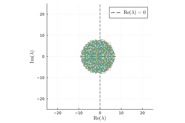
Each point in the plot is an eigenvalue of a matrix where $n=250$, $P=0.25$, $\sigma=1$, $d=1$. Notice the circular distribution of $\lambda$ with radius $\sqrt{nP\sigma^2}$.

Allesina and Tang matrices

Generate a matrices that follows Allesina’s and Tang’s assumptions:

1. Effects of species $i$ on species $j$ are typically not independent;
   • (a.) When there is competition between species $i$ and $j$, both $M_{ij}$ and $M_{ji}$ should be negative
   • (b.) When there is consumption (i.e. predator-prey), then when $M_{ij}>0$ we have $M_{ji}<0$
2. As a result, interactions are sampled in pairs from a bivariate distribution

Competition-mutualism matrix

function GenerateCompetitionMutualismMatrix(n::Int64, P::Float64, σ::Float64, r::Float64)
    # Generate community matrix that has the following constraints 
    # (i., 1a.) sign(Mᵢⱼ) = sign(Mⱼᵢ)  (i.e. mutualism if sign()>0 and competition otherwise)
    # (ii.)     Mᵢⱼ ~ p(0;σ)
    
    # Initialize random matrix 
    M = σ .* randn(n,n)
    #/ Force signs to be equal as per (1.)
    S = tril(sign.(M))
    # Remove random connections with prob. 1-P 
    S = S .* LowerTriangular(rand(n,n) .< (1-P))
    # Generate matrix with equal sign
    S = S .+ triu(transpose(S), 1)
    # Ensure (1.)
    M = abs.(M) .* S

    #/ Set diagonal elements
    M[diagind(M)] .= -r
    #/ Return
    return M
end

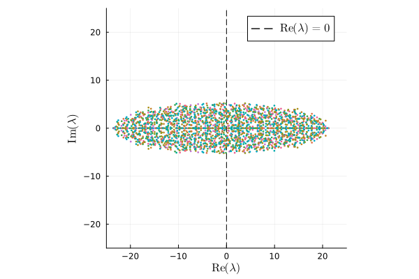
Competition and mutualism results in a horizontally stretched ellipse.

Predator-prey matrix

function GeneratePredatorPreyMatrix(n::Int64, P::Float64, σ::Float64, r::Float64)
    # Generate community matrix that has the following constraints 
    # (i., 1b.) sign(Mᵢⱼ) = -sign(Mⱼᵢ)  (i.e. predator-prey)
    # (ii.)     Mᵢⱼ ~ p(0;σ)

    # Initialize random matrix 
    M = σ .* randn(n,n)

    #/ Force signs to be opposite as per (1.)
    # Compute random lower triangular matrix to ensure opposite signs
    L = LowerTriangular(rand(-1:2:1,n,n))
    # Remove random connections with prob. 1-P 
    L = L .* (LowerTriangular(rand(n,n)) .< (1-P))
    # Generate matrix with opposite sign
    S = L .+ -1 .* triu(transpose(L), 1)
    # Force signs to be opposite as per (1.)
    M = abs.(M) .* S

    #/ Set diagonal elements
    M[diagind(M)] .= -r
    #/ Return 
    return M
end

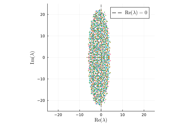
The predator-prey assumption leads to a vertically strechted ellipse.

Plots

We can plot the ‘distribution’ of eigenvalues simply by making scatter plots of all the eigenvalues for a few matrices. The above plots were generated with the following Julia module.

#/ Load libraries 
using Plots, LaTeXStrings, Random, LinearAlgebra
plot_font = "Computer Modern"
default(fontfamily=plot_font)

#/
function PlotEigenvalues!(M::Matrix{Float64}; pl=nothing)
    #/ Initalize plot 
    if pl === nothing
        pl = scatter(
            aspect_ratio=:equal, theme=:mute, seriestype=:scatter,
            xlabel = L"\textrm{Re}(\lambda)", ylabel=L"\textrm{Im}(\lambda)",
            xlims=(-25,25), ylims=(-25,25),
            xguidefontsize=11, yguidefontsize=11
        );
        pl = vline!(
            [0.], linestyle=:dash, color=:black, 
            label=L"\textrm{Re}(\lambda)=0", legendfontsize=11
        );
    end
    λ = eigvals(M)
    pl = scatter!(
        real(λ), imag(λ),
        label="", markersize=1.5, msc=:auto
    )
    return pl
end

Closing thoughts

The laws highlighted below show how useful random matrix theory can be in theoretical ecology. Of course, real-world community matrices are often not random and depend on a big swath of (external) factors. However, when communities are large, one can often extract distributions of the matrix components. If the characteristics of these distributions are, for example, close to those highlighted above, then one can already say a lot about the stability of such systems. It is also noteworthy to see that the actual distribution of elements of the distribution matrix does not matter much – as long as it is zero mean and has some finite variance. This ’enables’ many of these distributions to be used, and undoubtedly some real-world communities have precisely such distributions of their community matrix. Lately, however, more factors have been included in the community matrices that show the opposite of May’s results, namely that highly interconnected and diverse communities might actually be more stable. For now, the take-home message is that assuming simple mechanisms with ecological communities shows to lead to highly unstable communities. As we look around us, most communities are actually very stable, so other things must be at play that influence the long-term stability of ecosystems. Exciting!